Bio Fuels Optimization

Eighty percent of the cost of a gallon of fuel ethanol is the cost of the grain. Mother nature limits the yield to around 2.91 gallons of ethanol per bushel of grain, give or take a little.  Unfortunately, many fuel ethanol plants do not achieve any where near that yield at least not consistently. Given the current cost of corn a small consistent change in the yield can make the difference between profit and loss. Six Sigma methodology can and has been used to substantially increase fermentation yields.

Case Study 50 Million Gal/Yr Delta T Design Ethanol Plant

The plant was experienceing lower than desired yields (low 2.7s) and inconsistent performance. Using Six Sigma the plant found which of the hundreds of inputs are the critical few and which inputs are the trivial many.  By controlling the important inputs carefully the yield was maximized. After Six Sigma optimization plant achieved consistent yields in the high 2.8s.

The primary inputs to make fuel ethanol are grain, water, yeast and enzymes.  The outputs are ethanol, water, carbon dioxide, distillers grains and heat.  Beyond the primary inputs there are hundreds of process variables such as temperatures, flows, pH and many others. Which of these inputs have the largest impact on yield? Why do plants using the same corn the same water the same yeast and the same enzymes sometimes get 2.6 gal/bushel and sometimes they get 2.85 gal/bushel out of the same fermenter ?  In a 50 million gallon per year fuel ethanol plant at typical prices for corn and ethanol each 0.01 of yield can be worth hundreds of thousands of dollars per year in corn costs. See table.

Yield	Monthly Ethanol Production (gallons)	Monthly Corn Consumption (bushels)	Corn Cost ($/bushel)	Total Monthly Cost	Monthly Savings	Yearly Savings
2.73	4,300,000	1,575,092	$7.00	$11,025,641
2.74	4,300,000	1,569,343	$7.00	$10,985,401	$40,240	$482,875
2.75	4,300,000	1,563,636	$7.00	$10,945,455	$80,186	$962,238
2.76	4,300,000	1,557,971	$7.00	$10,905,797	$119,844	$1,438,127
2.77	4,300,000	1,552,347	$7.00	$10,866,426	$159,215	$1,910,580
2.78	4,300,000	1,546,763	$7.00	$10,827,338	$198,303	$2,379,635
2.79	4,300,000	1,541,219	$7.00	$10,788,530	$237,111	$2,845,327
2.80	4,300,000	1,535,714	$7.00	$10,750,000	$275,641	$3,307,692
2.81	4,300,000	1,530,249	$7.00	$10,711,744	$313,897	$3,766,767
2.82	4,300,000	1,524,823	$7.00	$10,673,759	$351,882	$4,222,586
2.83	4,300,000	1,519,435	$7.00	$10,636,042	$389,599	$4,675,183
2.84	4,300,000	1,514,085	$7.00	$10,598,592	$427,049	$5,124,594
2.85	4,300,000	1,508,772	$7.00	$10,561,404	$464,238	$5,570,850
2.86	4,300,000	1,503,497	$7.00	$10,524,476	$501,166	$6,013,986
2.87	4,300,000	1,498,258	$7.00	$10,487,805	$537,836	$6,454,034
2.88	4,300,000	1,493,056	$7.00	$10,451,389	$574,252	$6,891,026
2.89	4,300,000	1,487,889	$7.00	$10,415,225	$610,416	$7,324,993

 

To get this chart with your data i.e. your capacity, corn cost,current yield and potential savings please call James Frugé at 214-477-5141 or email at Jfruge@mac.com.

The Six Sigma method uses a road map for solving difficult problems such as yield optimization. The road map consists of Define, Measure, Analyze, Improve and Control, DMAIC.

 
DEFINE is important because it assures agreement on what the problem is, what the process boundaries are, how to measure the out come and who will be working on the project. Without Define, projects often suffer scope creep and are soon trying to "save the world".

The MEASURE step is where the team handles the problem of garbage in – garbage out (GIGO). Without data you can trust it is hard if not impossible to make good decisions. First, the team determines how well they can measure the output.  In the case of fermentation yield involves measuring how much corn was used in the fermenter batch, the ethanol in the final sample of fermentation and how many gallons are in the fermenter. Sounds simple in principle but can be difficult in practice. Many plants use High Pressure Liquid Chromatography (HPLC) to measure the amount of ethanol in the final or drop sample. How much of the variability from batch to batch is due to the variation of the process and how much is due to the measuring system, i.e. the HPLC? By analyzing samples that represent the range normally seen in the process in a statistical way the percent of variation caused by the measuring system (HPLC analysis) can be determined. In order for the measurement system to be good enough for process improvement work the variability caused by the measurement system should be less than 30% of the variability of the process.  The target is no more than 10%.  The same technique can be used to determine how well the solids i.e corn flour in the mash measurement system is.  Once these measurement systems have been proven to be “good” they can be used to calculate a batch yield, the Big Y.
The next part of Measure is to determine what are the inputs (little xs) to measure and how well they can be measured. A Process map is created by the team that identifies all of the inputs to the fermentation process. Then, a Measurement System Analysis (MSA) is performed on all of the inputs. In a Delta T design plant there are approximately 85 to 100 inputs that need to be checked out. Many times the MSA is just to make sure the measurement is done correctly and stored in the correct place in the data system. The assumption used is that all measurements are bad until proven other wise.  This step requires the efforts of operators, maintenance techs, management and just about everybody involved in running the process.
After making sure the data being used is “good” then data is collected on batches. It is important to not “experiment” at this time.  We are trying to find out how the normal operation of the plant looks like using “good” data. With all of the inputs captured and a batch yield to show how well or poor we did the Analyze phase can begin.

In ANALYZE we use Minitab to find the important input variables. Minitab is an intuitive statistical software package that has become the defacto standard for Six Sigma analysis.  Some people use a package called Jump® that works well also. There are Excel add-ons available but they are not as easy to use nor are they as powerful as Minitab.  First, a graphical analysis gives clues to which inputs have the greatest control over the yield and then statistical analysis determines which ones are significant. In most process with 85 to 100 inputs only three or four have a high impact on the variability of the process. Also, these critical few Big Xs are also unique to that particular plant. Even though all Delta T plants and all ICI plants are the same design there are differences that make each one unique.

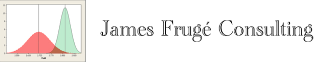
We are now ready for IMPROVE. After finding the critical few inputs , the big Xs, to confirm their importance and find out if there are any interactions between these inputs it is wise to run a Design of Experiments (DOE).  In a DOE you run the plant varying the important inputs in a specific way from their high value to their low value. Analysis of this data will confirm the importance of each variable and show how to best optimize the plant for maximum yield. Now, you set the important inputs at their optimum values and run the plant. After implementing the Six Sigma settings you should see something like this. (Individual chart of Yield before and after).

The CONTROL step is designed to make sure the improvements last. In order to improve the plant operations you must change what you were doing before.  Change is hard. There is a tendency to go back to the old ways.  The control plan is just a written plan for how we will be sure the important variables will be kept at their best values long term and how to detect when things have drifted off before it is too late.